How to Use Excel's One Way ANOVA to Solve Some Practical Statistics Problems - Statistics Homework Help
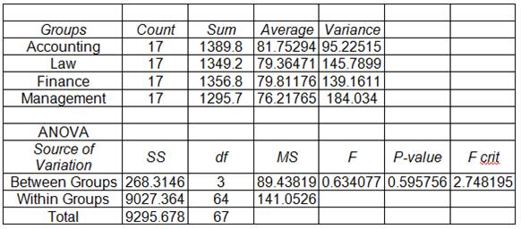
You collect the following salary figures for Master’s Level Students and their salaries after 2 years at work. You are interested in whether or not people with different degrees make more or less money. The data are analyzed using an ANOVA test with the following results:

1.) What are the null and experimental hypotheses?
Solution: The null and experimental hypotheses are
\[\begin{array}{cc} & {{H}_{0}}:{{\mu }_{A}}={{\mu }_{L}}={{\mu }_{F}}={{\mu }_{M}} \\ & {{H}_{A}}:\text{ not all the means are equal} \\ \end{array}\]
|
2.) Is there a significant difference between the four majors with regard to their salaries 2 years after graduation?
Solution: According to the values shown in the table, we fail to reject the null hypothesis, since the p-value is p = 0.595756, which is greater than the significance level 0.05. Therefore, we don't have enough evidence to claim that there is a significant difference between the four majors with regard to their salaries 2 years after graduation
3.) Consider a situation where the ANOVA showed that there WAS NOT a significant difference between the four majors. What would you recommend doing as a next step in the research to show that people with Accounting degrees make significantly more than graduates with Management-degrees?
Solution: To compare the mean salary of people with Accounting and Management degrees we need to use a t-test. We need establish a significance level, and then compute the critical t-value, in order to see if we reject or we fail to reject the null hypothesis.
4.) Consider a situation where the ANOVA showed that there WAS a significant difference between the four majors. A Tukey Critical Difference was calculated to be 4.8 for these data at 95% confidence. What does this statistic tell you about the data?
Solution: A Tukey Critical of 4.8 for these data at 95% confidence means that a pairwise comparison needs to exceed that value to be considered significant (with 95% confidence).
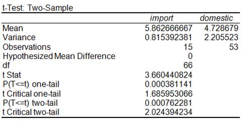
You want to know if there is a difference in price between imported and domestic beers. You go to your local supermarket and record the sales price and country of origin of 68 different beers. A t-test is run, the results of which appear below.

5.) Why would it be better to use a one-tailed test in this case?
Solution: We have the suspicion that import beer is more expensive than domestic beer. Therefore, we will take that as our experimental hypothesis. Therefore, our hypotheses would be
\[\begin{array}{cc} & {{H}_{0}}:{{\mu }_{IMPORT}}\le {{\mu }_{DOMESTIC}} \\ & {{H}_{A}}:{{\mu }_{IMPORT}}>{{\mu }_{DOMESTIC}} \\ \end{array}\]6.) You selected a one-tailed test, what are the null and experimental hypotheses (H0 and H1)?
Solution: As we stated in the previous part, we have
\[\begin{array}{cc} & {{H}_{0}}:{{\mu }_{IMPORT}}\le {{\mu }_{DOMESTIC}} \\ & {{H}_{A}}:{{\mu }_{IMPORT}}>{{\mu }_{DOMESTIC}} \\ \end{array}\]7.) In the beer price study, what is the critical value of t used in a one-tailed test?
Solution: The one-tailed critical t-value is \({{t}_{c}}=1.68595\), as shown in the Excel table above.
8.) Is there a significant difference between the price of domestic versus imported beers? What does this mean?
Solution: Yes, there is a significant difference. The t-statistics is equal to 3.66044, which is greater than the critical t-value. This means that we reject the null hypothesis, which means that the sample provides enough evidence to claim that there's a significant difference in price between domestic and import beers.
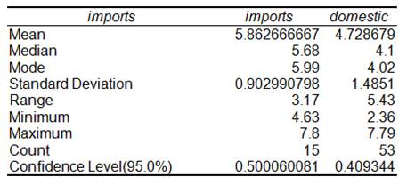
Descriptive statistics for both prices of beers were calculated. The results showed the following:

9.) What is the one BEST measure of central tendency (mean, median, or mode) to use for these data?
Solution: Considering the parametric nature of the comparison, the mean is the most suitable measure of central tendency to use for these data. The mean has very good properties, such as being an unbiased estimate to the population mean, and the standard deviation of the mean (standard error) converges to zero as the sample size gets bigger.
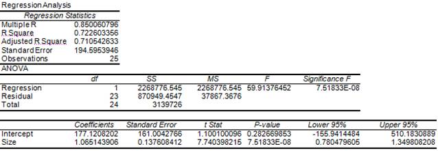
You are interested in the prediction of apartment rent from square footage. You sample 25 apartments in the Glendale area and record the apartment rent costs and square footage. When you put this into Excel, you get the following output:

10.) What is the regression equation for these data?
Solution: According to the Excel table above, the regression equation is given by
\[\hat{y}=177.1208202+1.065143906\times \text{Price}\]11.) How much of the variance in rent can be predicted by knowing the square footage?
Solution: We see that the
R Square coefficient is given by \[{{R}^{2}}=0.722603356\]which means that 72.2603356% of the variance in rent can be predicted by knowing the square footage.
12.) Is this a significant regression equation?
Solution: Using the table for Critical Values of the Pearson Correlation coefficient, the critical correlation for \(n=25\) is \({{r}_{c}}=0.505\), at the 0.01 significance level. Since the correlation for this model is 0.85, we conclude that the regression equation is significant, at the 0.01 significance level.
13.) What does this mean?
Solution: This means that there's exist a significant degree of linear association between the Rent and Size.
Wages in the construction industry average $11.90 per hour with a standard deviation of ![]() 10.50 per hour (z = -1.00)?
10.50 per hour (z = -1.00)?
Solution: Let $X$ the random wage. We need to compute
\[\Pr \left( X<10.5 \right)=\Pr \left( \frac{X-11.90}{1.40}<\frac{10.5-11.90}{1.40} \right)=\Pr \left( Z<-1 \right)\] \[=\Phi (-1)=0.158655\]where \(\Phi\) corresponds to the cumulative standard normal distribution. This means that 15.8655% of the workers make less than $10.5 per hour ]
15). What percent of workers make more than $15 per hour (z = 2.21)?
Solution: Similarly to the previous problem. We need to compute
\[\Pr \left( X>15 \right)=\Pr \left( \frac{X-11.90}{1.40}>\frac{15-11.90}{1.40} \right)=\Pr \left( Z>2.21 \right)\] \[ =1-\Pr \left( Z\le 2.21 \right)=1-\Phi (2.21)=0.013553\]This means that 1.3553% of the workers make more than $10.5 per hour.
You can send you Excel Stats homework problems for a Free Quote. We will be back shortly (sometimes within minutes) with our very competitive quote. So, it costs you NOTHING to find out how much would it be to get step-by-step solutions to your Stats homework problems.
Our experts can help YOU with your Statistics Assignments. Get your FREE Quote.
