How to Use SPSS to Conduct a Thorough Multiple Linear Regression analysis

The objective of this paper is to analyze the effect of the expenditure level in public schools and the results in the SAT. For this purpose, a dataset with demographic information from 50 states is provided. Other variables of interest provided that could have and effect on the mean SAT scores are the teacher’s salary, the average pupil/teacher ratio in public schools, and the percentage of all eligible students taking the SAT.

The research question is: “Which of these variables is a significant predictor for the SAT scores”

Introduction

The purpose of this paper is to analyze a dataset that involves information about the SAT scores obtained by public schools students and some other demographic variables, such as the public schools expenditures, teacher’s salary.

More specifically, we have information from 50 states that include the following variables:

o State: Name of state

o Exp: Current expenditure per pupil in average daily attendance in public elementary and secondary schools, 1994-95 (in thousands of dollars)

o Ratio: Average pupil/teacher ratio in public elementary and secondary schools, Fall 1994

o Salary: Estimated average annual salary of teachers in public elementary and secondary schools, 1994-95 (in thousands of dollars)

o Perc: Percentage of all eligible students taking the SAT, 1994-95

o Verb: Average verbal SAT score, 1994-95

o Math: Average math SAT score, 1994-95

o Total: Average total score on the SAT, 1994-95

The main purpose of this paper is to analyze the influence of these variables in the average total score on the SAT. A regression analysis will be used to determine which variables are significant predictors of Total.

From a theoretical point of view, all these variables seem to have an influence on Total, and it makes sense to include them on the model.

For some of the variables, the directionality of the relation is predictable. For instance, it is expected that there is a positive relationship between Exp and Total (it is expected that more expenditure in public schools will bring higher scores). Same thing occurs with the variable Salary, which intuition suggests that there is a positive relationship with total.

Nevertheless, it is not clear whether these relationships are significant or not. In fact, only by applying appropriate statistical analysis that significance of our model can be assessed.

The data are appropriate for this study, and a regression analysis is suitable in this case for these quantitative variables. The sample size is not too large, but it a little bit above the bare minimum for obtaining meaningful statistical results. A larger sample size, though, would have been preferred.

Since the variable Total is the sum of Math and Verb, only one of those variables should be included to avoid multicollinearity problems. Arbitrarily, Verb will be dropped.

Method

The data provided is suitable for statistical analysis. The appropriate procedure is Multiple Linear Regression. The idea is to find a linear model that is significant and fits the data appropriately.

The first step of the analysis is to verify the appropriateness of the linear model, with scatterplots and a correlation matrix. If a linear regression is not suitable, some non-linear models should be attempted.

Among the research hypotheses that will be tested, the first one is the significance of the whole model (through the ANOVA table, F-test).

After the significance of the whole model is assessed, it is necessary to assess the significance of each individual predictor. If not all the predictors are significant, the next task is not find the “best” model: this is, a model that has mainly significant predictors and it explains the most amount of variation of the response variable. For this step a process called Stepwise Regression will be used. The main framework for the calculations will be the statistical software SPSS.

SPSS Regression Results

First of all, the linearity of the model needs to be assessed. The following chart shows a matrix scatter plot:

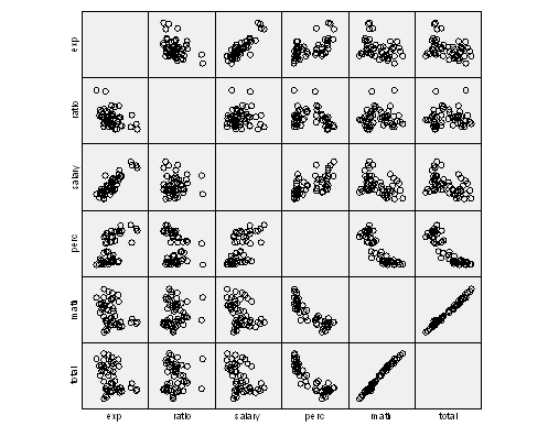
The plot above shows that at least some variables are significantly linearly related to Total. The variables with the clearest association are Perc and Math. The others show certain degree of association, but it is not clear.

Below, the correlation matrix is shown:

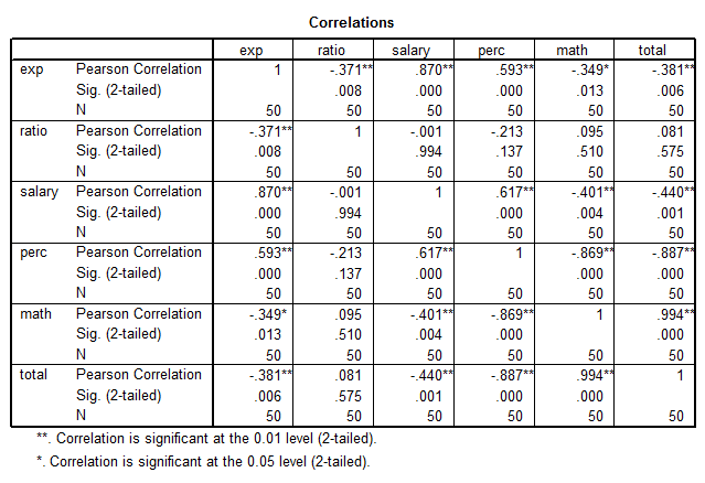
The correlation matrix shows some extra information. In fact, all of the predictors are significantly linearly related to Total, except for Ratio. But also, several predictors are linearly related to other predictors, which suggest a possible problem with multicollinearity.

This implies that a linear regression makes perfect sense, but one factor to be careful of is the possible redundancy in the data (multicollinearity)

Descriptive Statistics:

The following box-plots are presented

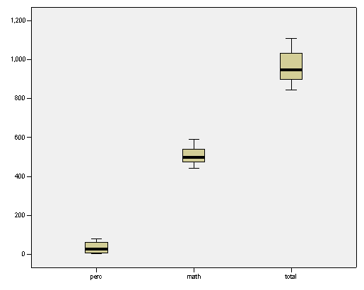
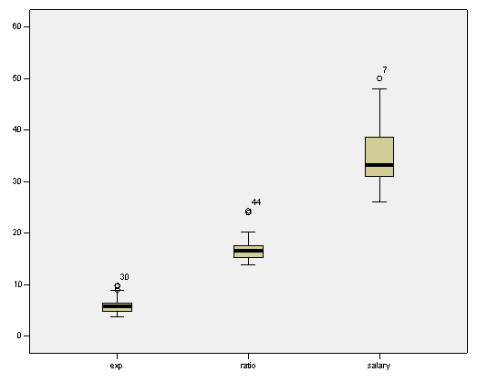
The plots above show the presence of a few outliers, but in the context of the data set those data seem to be legitimate, so no data will be erased.

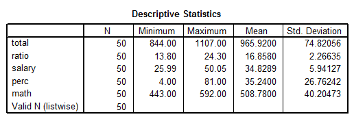
The following are the descriptive statistics for the relevant variables:

Regression Results:

The following tables from SPSS show the results from a regression analysis:

• The table above shows that the correlation coefficient is R = 0.995, and the adjusted R² is 0.989, which indicates that 98.9% of the variation in Total is explained by this model

• The table above shows that the model is significant overall (p = 0.000), this means that at least one variable in this model is significant. This is not surprising considering the type of scatterplot found.

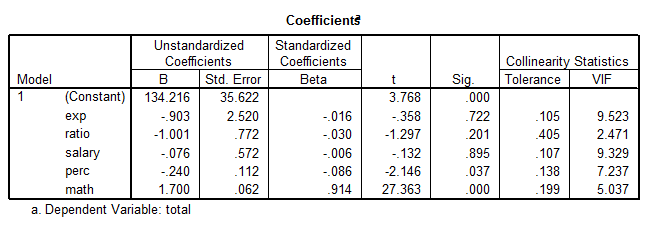
The table above shows that not all the predictors are significant. In fact only Math (p = 0.000) and Perc (p = 0.037) appear to be significant, whereas the rest is not. Nevertheless, the VIF factors are a bit high suggesting some multicollinearity complications.

The results of a stepwise regression are shown below:

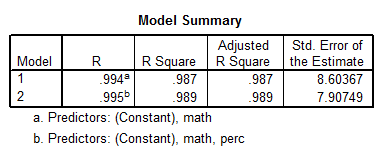
The table above shows that Exp, Ratio and Salary can be dropped out of the model, and for the most part the quality of the model is the same. In fact, the adjusted R² is 98.9%. Also, the multicollinearity problems disappeared for the most part. The best model is

\[Total = 113.505 + 1.694Math - 0.268Perc\]

Regression Assumptions:

Now the regression assumptions need to be verified for this best model found. First of all, the adequacy of the linear model is clear from the original multiple scatterplot. Also, the VIF are less than 5, which indicate in practicality no multicollinearity problems.

For the normality of residuals, the following histogram is presented:

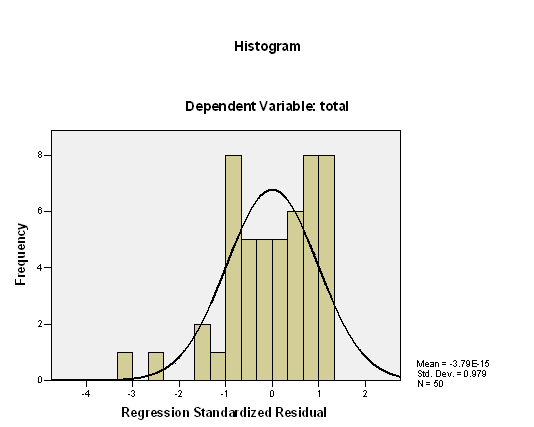
There is no clear sign of a violation of normality, except that the data look a bit non-symmetrical (left-skewed).

In terms of the homogeneity of the variance, the following plot is presented:

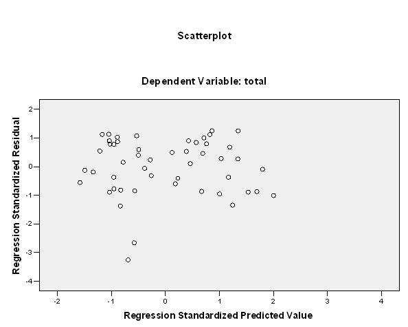
The plot above doesn’t show a major trend going on, so there is no clear evidence of heteroskedasticity.

In other words, for the most part, the assumptions for a linear regression are satisfied.

Conclusions

The answer to the research question seems to negative. The variable Exp doesn’t seem to be a significant predictor for the model. Exp does present some degree of linear association with the response variable Total, but in the context of the model, the same amount of variance can be explained without it. Same happens with Salary and Ratio, which contrary to what the intuition indicates don’t play a significant role in the model.

Given the dataset provided, the best model is

\[Total=113.505+1.694Math-0.268Perc\]

This model provides a higher adjusted R² coefficient and a smaller standard error of the estimate than the full model with all the original predictors, and the two variables are significant. Hence, this model is the preferred one.

For this model, the regression assumptions seem to be satisfied.

• Alternative Model

In regression analysis, it is very important to following theoretical considerations at the time of including the variables in the model. Sometimes, even if the data don’t support the presence of certain variable in the model, still due to strong theoretical/empirical reasons we may have a reason to include that variable (Let’s recall that if a variable doesn’t seem to be significant, that can also be due to some other problems, like violation of some of the regression assumptions)

We are going to test one more model, which includes Exp and Perc as predictors. The output from SPSS is shown below:

The model is
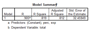
\[Total=993.832+12.287Exp-2.851Perc\]

We observe that this model is significant (p = 0.000), and each predictor is significant as well. But this model doesn’t explain nearly as much variation as the best model found below. In fact, now we have that \(Adj.\,{{R}^{2}}=0.812\), as opposed to \(Adj.\,{{R}^{2}}=0.989\) found for the best model above.

This model is still reasonably good, and it can be considered as a viable model is empirical considerations require it.

---

You can send you Stats homework problems for a Free Quote. We will be back shortly (sometimes within minutes) with our very competitive quote. So, it costs you NOTHING to find out how much would it be to get step-by-step solutions to your Stats homework problems.

Our experts can help YOU with your Stats. Get your FREE Quote. Learn about our satisfaction guaranteed policy: If you're not satisfied, we'll refund you. Please see our terms of service for more information about this policy.

Contact Us!