How to Use SPSS to run a linear regression and a One-Way ANOVA.

CASE STUDY: REGRESSION AND ANOVA

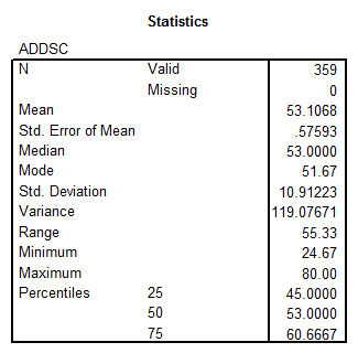
• ADDSCC: This variable corresponds to a continuous variable, with the ratio level of measurement. We obtain the following descriptive statistics from SPSS

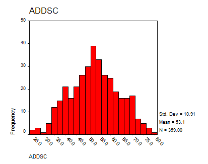
The distribution of the variable is shown below in the form of a histogram:

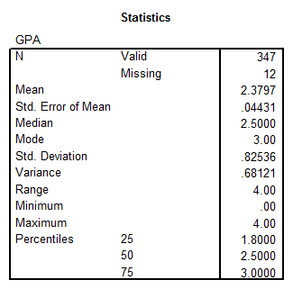
• GPA: This variable corresponds to a continuous variable, with the ratio level of measurement. We obtain the following descriptive statistics from SPSS

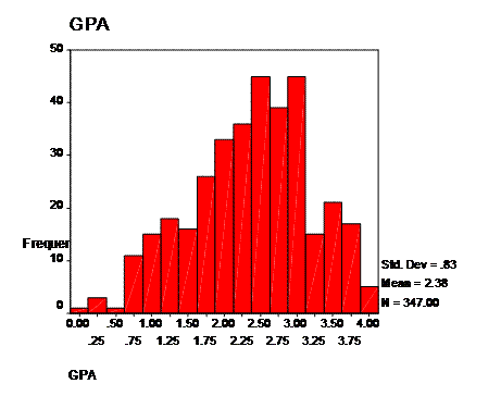
We have the histogram:

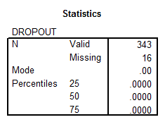
• DROPOUT: This variable corresponds to a discrete variable, with the nominal level of measurement. The descriptive statistics are shown below

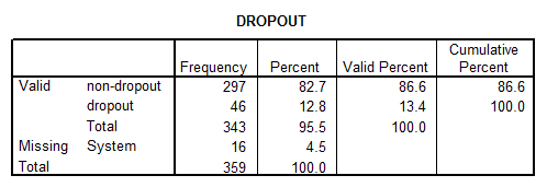
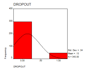
The distribution looks like:

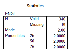
• ENGL: This is a discrete variable with the nominal level of measurement. The descriptive statistics we obtain with SPPS are

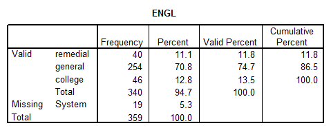
The distribution is given by

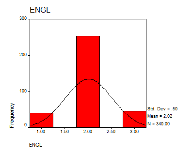
• GENDER: This is a discrete variable with the nominal level of measurement. The descriptive statistics are

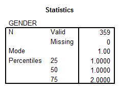
The distribution is shown below:

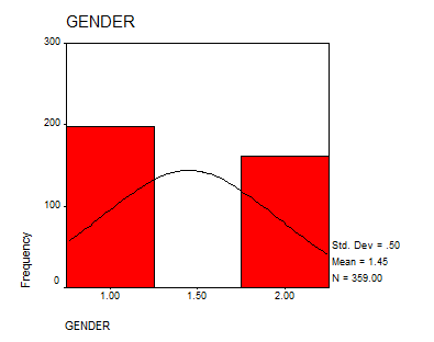
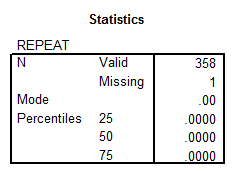
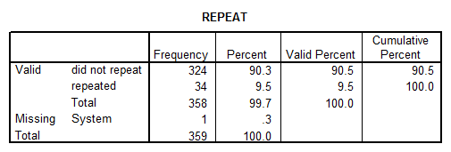
• REPEAT: This is a discrete variable with the nominal level of measurement. The basic descriptive statistics are

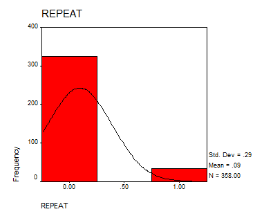
The histogram looks like:

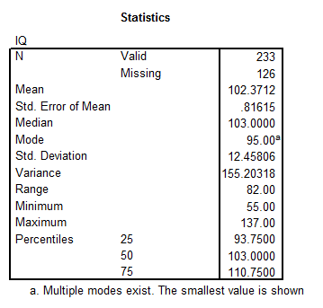
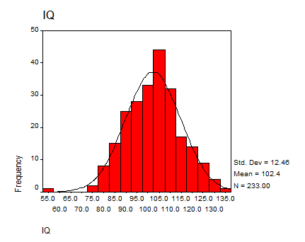
• IQ: This variable corresponds to a continuous variable with the ratio level of measurement. The descriptive statistics we find with SPSS are

The histogram is given by:

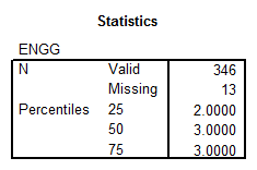
ENGG: This variable corresponds to a discrete (ordinal level of measurement) variable. The basic statistics are

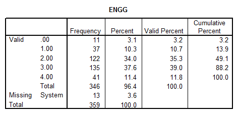
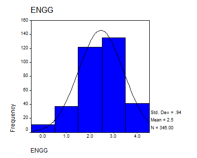
The distribution looks like:

• SOCPROB: This variable corresponds to a discrete variable, with the ordinal level of measurement. The descriptive statistics are

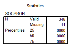
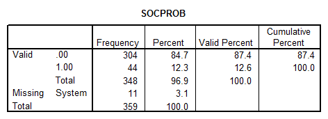
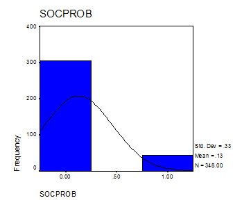
The distribution looks like:

3A. INFERENTIAL PROCEDURES

We analyze the degree of linear correlation between GPA and ADDSC using SPSS:

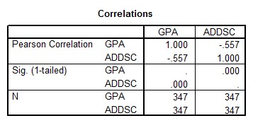
The correlation coefficient is equal to

\[\rho =-0.557\]

which shows a significant level of linear association between GPA and ADDSC, based on the p-values shown in the table. In order to analyze the normality of these two variables, we proceed in the following way:

ADDSC: We are going to test

\[\begin{align} & {{H}_{0}}:\text{ ADDSC has a normal distribution} \\ & {{H}_{A}}:\,\text{ADDSC has not a normal distribution} \\ align="center">\end{align}\]

The results of the Kolmogorov-Smirnov test are shown below:

The p-value is equal to \(p = 0.200\), which shows that we cannot reject the null hypothesis of normality. This implies that there is not enough evidence to reject the normality assumption

GPA: We are going to test

\[\begin{align} & {{H}_{0}}:\text{ GPA has a normal distribution} \\ & {{H}_{A}}:\,GPA\text{ has not a normal distribution} \\ \end{align}\]

The results of the Kolmogorov-Smirnov test are shown below:

The p-value is equal to \( p = 0.000\), which means that we reject the null hypothesis of normality. There is enough evidence to reject normality of GPA

• Now we perform a Linear Regression analysis:

The adjusted

R Square

coefficient is equal to

\[\text{Adj }{{R}^{2}}=\text{0}\text{.308}\]

which means that only 30.8% of the variance of the dependent variable (GPA) is explained by the linear regression.

• ANOVA analysis:

The table shows that the model is significant overall (\(p=0.000\)).

The regression coefficients are

The p-value shows that ADDSC is a significant predictor (\(p=0.000\)), which means that the Regression Equation is

\[\hat{y}=4.653-0.0430x\]

3B. DIFFERENCE BETWEEN GROUPS

We run a t-test to determine if there is any difference between the mean GPA of dropouts and non-dropouts. In other words, we are going to test the following hypotheses

\[\begin{align} & {{H}_{0}}:{{\mu }_{1}}={{\mu }_{2}} \\ & {{H}_{A}}:\,{{\mu }_{1}}\ne {{\mu }_{2}} \\ \end{align}\]

where \({{\mu }_{1}}\) represents the mean GPA of dropouts, and \({{\mu }_{2}}\) represents the mean GPA of non-dropouts.

The following are the results using SPSS.

• The table shows that Levene’s Test is not significant, which means we can assume equal variances.

• The p-value for the t-test is equal to $p=0.000$. That means that we have enough evidence to claim that non-dropout students have higher GPA than dropout students.

3C. DIFFERENCE AMONG GROUPS

We need to test the following hypotheses:

\[\begin{align} & {{H}_{0}}\text{: }{{\mu }_{{{G}_{1}}}}={{\mu }_{{{G}_{2}}}}\text{=}{{\mu }_{{{G}_{3}}}}\text{ } \\ & {{H}_{A}}\text{: the means are not equal}\, \\ \end{align}\]

We use Analysis of Variance, ANOVA, to determine whether there is or not a difference between the group means.

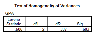
Levene's Test shows that we can consider the variances to be all the same, since p = 0.603, which is not less than the significance level.

The ANOVA analysis shows evidence that there is enough evidence to claim that not all the means are the same.

• Now that we know that there is a difference between the means, we need to perform a Post-Hoc analysis, which is shown below:

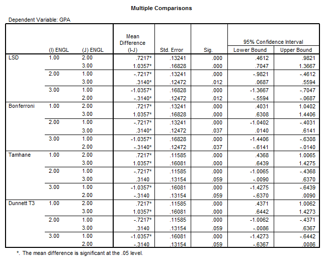
Using the LSD test, we conclude that

• The mean of the group 1 is greater than the other group means.

• The mean of group 2 is higher than the mean of group 3.

3D. INDEPENDENCE OF CATEGORICAL VARIABLES

We need to test the following hypotheses

\[\begin{align} & {{H}_{0}}\text{: ''Gender''}\text{ and ''Repeat'' are independent} \\ & {{H}_{A}}:\,\text{ ''Gender''}\text{ and ''Repeat'' are NOT independent} \\ \end{align}\]

We have the following crosstabulation:

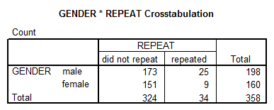
Using the Chi-Square Test for independence (the variables are categorical)

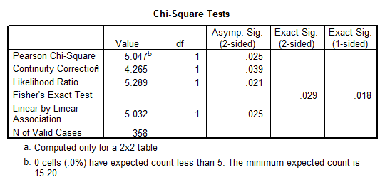
• The Chi-Square is significant, with a p-value of \(p = 0.025\), which implies that we have GENDER and REPEAT are dependent, at the \(\alpha =0.05\) significance level.

3E. EXTRA RESEARCH QUESTION

Is the linear association between IQ and GPA statistically significant?

Using SPSS: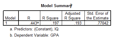

The correlation coefficient is equal to

\[r=0.443\]

which indicates a significant level of linear association between GPA and IQ. This association is rather weak though, given that the R Square coefficient is \({{R}^{2}}=0.197\), which means that only 19.7% of the variation in the GPA is explained by the IQ variable.

The ANOVA analysis shows that model is significant overall, with a p-value equal to \(p=0.000\). The coefficients are:

The table shows that IQ is a significant predictor of GPA (\(p=0.000\)). The Regression Equation is equal to

\[\hat{y}=-7.22+0.03067x\]

---

You can send you Stats homework problems for a Free Quote. We will be back shortly (sometimes within minutes) with our very competitive quote. So, it costs you NOTHING to find out how much would it be to get step-by-step solutions to your Stats homework problems.

Our experts can help YOU with your Stats. Get your FREE Quote. Learn about our satisfaction guaranteed policy: If you're not satisfied, we'll refund you. Please see our terms of service for more information about this policy.

Contact Us!